


Introduction
Arctica islandica (Linnaeus, 1767) is a boreal bivalve with an expansive range in the northern hemisphere that also has the unique capacity for individuals to survive for centuries. The last extant species of the family Arcticidae, A. islandica (i.e. ocean quahog) is endemic to the Arctic and Atlantic oceans and currently inhabits shelf waters from Norway to the British Isles and Iceland, the Baltic and White Seas, and from Newfoundland to Cape Hatteras (Cargnelli et al., Reference Cargnelli, Griesbach, Packer and Weissberger1999; Dahlgren et al., Reference Dahlgren, Weinberg and Halanych2000; Butler et al., Reference Butler, Richardson, Scourse, Witbaard, Schöne, Fraser, Wanamaker, Bryant, Harris and Robertson2009; Gerasimova & Maximovich, Reference Gerasimova and Maximovich2013). This species is found at depths between 25–61 m and occurs at an average depth of 42 m in the western Mid-Atlantic (Merrill & Ropes, Reference Merrill and Ropes1969), but depth and distance offshore are regional responses to bottom water temperatures (Franz & Merrill, Reference Franz and Merrill1980; Dahlgren et al., Reference Dahlgren, Weinberg and Halanych2000).
In addition to the fascinating longevity exhibited by A. islandica, this species represents an important fishery in the western Atlantic. Fishery landings in the USA are divided into a Gulf of Maine fishery that targets younger and smaller clams (i.e. mahogany clams), and the southern fishery that targets larger clams (>80 mm shell length) that spans Cape Hatteras in the south to Georges Bank in the north-east (Merrill & Ropes, Reference Merrill and Ropes1969; Franz & Merrill, Reference Franz and Merrill1980; Dahlgren et al., Reference Dahlgren, Weinberg and Halanych2000). Georges Bank is considered a separate management area within the southern fishery due to the extreme distance offshore and separation from the contiguous southern fishery by the Great South Channel (NEFSC, 2017). Paralytic shellfish poisoning closed Georges Bank for surfclam and ocean quahog commercial harvests in 1989 and this area remained closed until recently reopened to these fisheries in 2013 (DeGrasse et al., Reference DeGrasse, Conrad, DiStefano, Vanegas, Wallace, Jensen, Hickey, Cenci, Pitt, Deardorff, Rubio, Easy, Donovan, Laycock, Rouse and Mullen2014; NEFSC, 2017). Accordingly, the Georges Bank population can be considered quasi-virgin (i.e. unfished) due to restricted commercial accessibility and minimal annual ocean quahog landings (less than 0.5% of total stock landings between 2000–2016, with no reported landings prior to 2000) (NEFSC, 2017).
Arctica islandica is managed in the USA by means of length-based population models, a stark contrast to the age-based models applied to many other fisheries. The extreme variability in age-at-size (Pace et al., Reference Pace, Powell, Mann and Long2017a, Reference Pace, Powell, Mann, Long and Klinck2017b) makes producing reliable age estimations from size difficult when using age-length keys (ALK) or growth curves, thereby limiting the use of age-based models. In addition, the longevity of this species poses particular management challenges because a recruitment index is unavailable over a time frame consistent with the longevity of the animal, thereby creating uncertainty as to sustainable yield and the time frame required for rebuilding should the stock be overfished. Historical presumptions for A. islandica include prolonged lapses in recruitment to sustain such longevity (Powell & Mann, Reference Powell and Mann2005), but this conclusion was based on recent recruitment data from the southernmost portion of the Western Atlantic range; a longer-term recruitment time series cannot be predicted without age-frequency data. Pace et al. (Reference Pace, Powell, Mann and Long2017a) identified that extremely large sample sizes are likely required to provide adequate resolution in the A. islandica ALK to develop a suitable, population-scale age frequency.
A further impediment to understanding A. islandica population dynamics is the differential growth rates of male and female A. islandica (Ropes et al., Reference Ropes, Murawski and Serchuk1984; Fritz, Reference Fritz1991; Thorarinsdóttir & Steingrímsson, Reference Thorarinsdóttir and Steingrímsson2000). Sexual dimorphism is rare in bivalves, excepting the protandrous taxa. The degree of sexual dimorphism in A. islandica may require sex-specific age-length keys. Sexual dimorphism often co-occurs with sex-dependent mortality rates, whereby distinct age frequencies may also exist and might influence both length- and age-based models (Wilderbuer & Turnock, Reference Wilderbuer and Turnock2009; Maunder & Wong, Reference Maunder and Wong2011).
The objectives of this study are to address gaps in the current fishery assessment models by examining the ability to produce age-based model parameters including a reliable age-length key to estimate ages, estimates of mortality and longevity, evaluating proxies for recruitment indices such as age-frequency distributions, and determining whether sex-specific considerations need to be made. Georges Bank was chosen for this analysis as it represents a nearly virgin stock, thus providing proxy baseline data on the population dynamics of this species and potential recruitment trends over time in the western Mid-Atlantic region.
Materials and methods
Sample collection
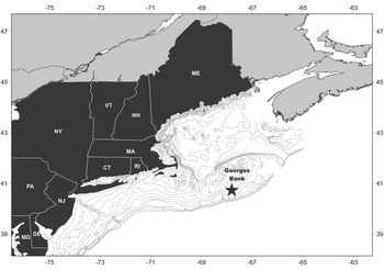
Two field samples were collected for this project: a length sample and a shucked sample. Each sample was obtained from approximately the same site (40.72767°N 67.79850°W) at a depth of ~72 m (Figure 1). This site falls within the new federal survey stratum 9Q (Jacobson & Hennen, Reference Jacobson and Hennen2019). Both samples are unbiased representations of the population in that no subsampling occurred. The length sample was collected in 2015 for a previous Arctica islandica age study (see Pace et al., Reference Pace, Powell, Mann and Long2017a, Reference Pace, Powell, Mann, Long and Klinck2017b) by a hydraulic clam dredge employed by both the fishery and federal survey (Hennen et al., Reference Hennen, Mann, Charriere and Nordahl2016). Commercial fishing gear, including the survey gear used for this collection, targets, and is therefore highly selective for, animals greater than ~75 mm (Hennen et al., Reference Hennen, Mann, Charriere and Nordahl2016; NEFSC, 2017); selectivity falls rapidly for sizes <60 mm. To limit uncertainty imposed by a correction for selectivity, this study focused on the highly selected size classes ≥75 mm. Analysis, thusly, focuses on the length classes pertinent to fishery stock demographics and to the federal stock assessment programme. The 2015 length sample included shell lengths for 2778 Arctica islandica that were used to construct the length frequency.

Fig. 1. Location of the 2015 length- and 2017 shucked-sample sites (star) on Georges Bank.
In 2017, a more intensive age analysis was conducted to age more A. islandica per size class than the studies of Pace et al. (Reference Pace, Powell, Mann and Long2017a, Reference Pace, Powell, Mann, Long and Klinck2017b). A differential sampling protocol was used so that sufficient animals of a range of size classes could be obtained for ageing. The 2017 shucked sample was collected from the same location as the 2015 length sample which permitted reutilization of the 2015 length sample. The 2017 shucked sample was collected with a Dameron–Kubiak (DK) dredge that allowed variable bar spacing to collect animals <80 mm and increase sample sizes for smaller animals available to the fishery (Hennen et al., Reference Hennen, Mann, Charriere and Nordahl2016). Although animals between 70–74 mm in shell length were not included in the 2015 length sample, these animals were retained by the DK dredge and included in the shucked sample so no age data would be omitted for such a data-poor species. Multiple 5-min tows from the same site were required to obtain sufficient numbers of animals for the large, rare size classes. Clam sexes were determined using gonadal tissue samples that were examined microscopically for the presence of sperm or eggs. The 2017 shucked sample included a total of 706 clams measured for shell length, sexed, shucked to remove all tissue, and the shell valves retained in dry storage for subsequent ageing.
Length frequency
To obtain an accurate representation of Georges Bank population demographics, the 2015 length sample was adjusted using a dredge selectivity coefficient (see table 15 in NEFSC, 2017). This selectivity coefficient was derived by federal assessment biologists across 20 sites within the US Mid-Atlantic A. islandica stock management area for the survey dredge employed by this study to collect the length sample.
Sex data were not collected for the 2015 length sample; therefore, the length sample was divided into male and female length frequencies by use of sex proportion at size from the 2017 shucked sample (N = 706) for each 1-mm size class. The population length frequency is the unsexed 2015 selectivity-adjusted length sample and included 3159 animals, that was subsequently divided to produce the female (N = 1470) and male (N = 1689) length frequencies.
Age frequency
The 2017 shucked sample was divided into 5-mm size classes and 100 animals per size class were chosen for ageing to create the age sample. These 100 animals consisted of ~50% randomly selected males and 50% randomly selected females (if available) to prevent a sex bias in numbers of aged animals per size class. All animals were aged for rare size classes that contained less than 100 animals. Sample processing methods were consistent with Pace et al. (Reference Pace, Powell, Mann, Long and Klinck2017b) and ageing techniques were consistent with Pace et al. (Reference Pace, Powell, Mann, Long and Klinck2017b) and Hemeon et al. (Reference Hemeon, Powell, Robillard, Pace, Redmond and Mann2021). Animals selected for ageing constituted the age sample and included true age and length data. This dataset was quality controlled using a second age reader for precision, bias and error frequency error analyses (Hemeon et al., Reference Hemeon, Powell, Robillard, Pace, Redmond and Mann2021). A total of 615 animals were aged, including 306 females and 309 males (Table 1).
Table 1. Summary of all data used to describe the Georges Bank population including the number aged at length (age-length), length-frequency, and age-frequency datasets

Population age-frequency was created with a unique age-length key, so population sample number is not the sum of male and female sample numbers. Each age-frequency sample (male, female, population) is subject to individual rounding procedures.
Age-length keys (ALK) are probability arrays that describe the probability of different animal ages at a given length and are created by amassing many samples with associated age and length data (Mohn, Reference Mohn1994; Harding et al., Reference Harding, King, Powell and Mann2008; Stari et al., Reference Stari, Preedy, McKenzie, Gurney, Heath, Kunzlik and Speirs2010). Unique ALKs were created in this study for the population, female and male groups using the age sample binned into 5-mm length size classes. Following ALK construction using the 2017 age sample, the corresponding 2015 length frequency (population, male, female) was applied to the analogous ALK to produce 2015 population, female and male estimated age frequencies. Resulting fractions in the age frequency were rounded up to whole individuals to prevent the elimination of a fraction of an animal due to rounding which would remove data for rare age classes. Consequently, male and female age frequencies do not sum to the number of animals in the population age frequency because each age frequency was created independently from unique ALKs and unique length frequencies. The population age frequency included 3248 animals, female age frequency 1525 animals and male age frequency 1742 animals (Table 1).
Longevity and mortality
Georges Bank is a site with no historic, and limited contemporary, commercial harvest of Arctica islandica. Consequently, total mortality is assumed to be equivalent to natural mortality (ocean quahog bycatch from the Atlantic surfclam fishery is also considered negligible at Georges Bank; see NEFSC, 2017). The descending right tails of the age frequencies were used to estimate mortality and longevity by linear regression of the natural log of the age frequencies (e.g. Ricker, Reference Ricker1975; Hoenig, Reference Hoenig2005; Kilada et al., Reference Kilada, Campana and Roddick2007; Ridgway et al., Reference Ridgway, Richardson, Scourse, Butler and Reynolds2012). Data were collapsed into 10-y age classes for this analysis to remove extreme noise in the data. The descending left tail of the age frequency is likely a product of low selectivity to the commercial dredge rather than low abundance and was not used to estimate mortality. Therefore, linear regression was evaluated for age frequencies greater than 100 y and represented 49% of the population and male age frequency data, and 48% of the female age frequency data. The x-intercept denoted the longevity estimate and slope represented the mortality rate.
Statistics
Frequency distributions
Tests to analyse significant differences between male and female length- and age-frequency distributions included the Kolmogorov–Smirnov (KS) (Conover, Reference Conover1980), Wald–Wolfowitz Runs (Conover, Reference Conover1980) and Anderson–Darling (AD) (Pettitt, Reference Pettitt1976; Engmann & Cousineau, Reference Engmann and Cousineau2011) tests at both 0.05 and 0.01 significance levels. The Runs test identifies systematic shifts in the distribution and, as used here, is designed to identify limited crossings of frequency distributions as might occur if male and female growth rates differed. The KS test and AD test compare the deviation between two frequency distributions, with the KS test being more sensitive to deviations in the central portion of the distribution and the AD test to deviations at the tails of the distribution. The AD test was included due to the rarity of old animals in the age-frequency distributions (distribution tails) and the KS test was included to identify episodic recruitment and mortality events (distribution central tendencies). Critical values were obtained from Conover (Reference Conover1980) for the KS and Runs tests and from Rahman et al. (Reference Rahman, Pearson and Heien2006) for the AD test. The KS test and the AD test were operated as two-sample, two-tailed tests, and rows without data outside the range of frequency data (leading and trailing double zeros) were deleted. For the KS and AD tests, the number of observations (n) was defined as the number of classes instead of the sum of the data supporting the classes, as doubling or halving the number collected and measured would not have materially changed the cumulative frequency distribution. The Runs test was operated as a one-sided test to evaluate only the ‘low’ condition, by which the distributions failed to cross each other at a minimal frequency expected by chance. In many cases, the total number of males and females of a length frequency differed due to sex ratios at size. To exclude a sex-ratio bias for the Runs test, the number of males and females was represented proportionately by length or age class.
In addition to the standard KS, Runs and AD tests listed above, a separate round of distribution test statistics were applied to modified versions of the distribution data used in the previous analysis. These modifications address the heavily right-skewed age frequencies that contain many instances of low to zero numbers of individuals in the tails of the distribution which can overly influence statistical evaluation of the distribution as a whole. Accordingly, in the spirit of the same approach used commonly in chi-square, the age and length classes with small numbers were also compressed by amalgamating adjacent classes. Unlike chi-square (e.g. Conover, Reference Conover1980), no standard rule is available to amalgamate class groups. In the present case, the median number in all classes was used and adjacent classes amalgamated until the number of individuals reached or exceeded this value. One of the two datasets (i.e. male or female) is required to designate the median to be applied to both datasets. That dataset herein is referred to as the reference dataset and the analysis is completed twice with each dataset assigned as the reference dataset. Once data were grouped into new frequency bins using the median, the KS, Runs and AD analyses were again performed, and this new type of analysis is herein referred to as median bin modification.
Age-length keys
To test the reliability of the male and female age-lengths keys (ALKs), 50 Monte-Carlo simulations were performed for each sex by randomly sampling with replacement from the true age-length data and new age-length keys were created for each simulation. Random samples included the same number of animals aged per 5-mm size class as the true dataset in order to represent the real ageing intensity, thereby preventing oversampling of rare size classes. The corresponding sex-specific length frequency was applied to the new ALK produced by each of the 50 simulations (herein referred to as the base simulations), and the resulting female and male age frequencies were tested for significant differences from the true age frequency by the KS, AD and Runs statistical tests.
A second set of 50 Monte Carlo simulations was completed in the same manner listed above, but new simulated ALKs were applied to the opposite sex length frequency and produced an additional 50 age frequencies per sex. These new age frequency distributions (herein referred to as the substituted simulations) were tested against the true age frequency using the KS, AD and Runs tests. If no significant difference exists between ALKs when the same length frequency is applied, the proportion of significant differences across 50 simulations would be the same for both the base and substituted simulated age frequencies. The proportion of base simulations with significant test results from the true age frequency was deemed the expected proportion of differences from a sampled population. A one-sample approximate binomial test for large samples (i.e. proportions test; R Core Team, 2018) was used to compare the proportion of significantly different substituted simulations from the expected proportion of significantly different base simulations (e.g. if the base simulations were statistically different from the true age frequency x/50 times, this would be the expected proportion; the proportion of significantly different substituted simulations would be compared with the expected proportion using a binomial test). If the ALKs were similar between sexes, substitution of the ALK applied to the same length frequency would create similar age frequencies to those of the true age frequencies and base simulations; whereas, if the ALKs were significantly different between sexes, the substituted ALKs would create different age frequencies when compared with the true age frequencies and the base simulations.
Sex ratios
Sex ratios were expected to be at one-to-one proportions across size classes. A one-sample binomial test (approximate binomial test for large samples (total N > 30), and one-sample exact binomial test for small samples (total N < 30); Conover, Reference Conover1980) (R Core Team, 2018) was used to evaluate a proportional sex ratio hypothesis for sex differentiated animals in the shucked sample (N = 706). A two-tailed analysis was performed to identify if the ratio is significantly different than what would be expected by chance (expected proportion of 0.5) and, if significant, a one-tailed test was used to identify if the ratio of females is less than or greater than what would be expected by chance.
Comparison of the means
Distribution statistics were applied to test differences in the shapes and spread of the length- and age-frequency data, likewise, mean statistics were applied as a secondary analysis to test whether male and female datasets represent the same population. Male and female length frequency data were tested for significant difference with a Mann–Whitney U test using R base statistics functions (population data omitted from this analysis as it is not an independent or paired dataset) (R Core Team, 2018).
Age data are positively skewed and therefore ranked (use of mean ties) before use in ANOVAs with alpha = 0.05 (it should be noted that an independent analysis that compared both parametric (raw ages) and non-parametric (ranked ages) tests produced similar results). Age composition between size classes were evaluated by type III one-way ANOVA and Tukey post-hoc tests, and age composition by sex between size classes were evaluated with a type III one-way multiplicative ANOVA model (R Core Team, 2018). Age compositions between population, female and male frequencies were assessed by type III ranked one-way ANOVA (R Core Team, 2018).
Results
Length frequency
The 2015 length frequency was divided into male and female length datasets by applying a sex proportion at size (1 mm) to the original dataset. Numbers at size, by sex used to create these proportions are shown in Table 2. The Georges Bank population length frequency had a mean length of 93 mm (SD = 7) and ranged from 76–116 mm (Figure 2). The central tendencies for the female length frequency (M = 96 mm, SD = 6; median = 95 mm) were larger than central tendencies for the male length frequency (M = 91 mm, SD = 6; median = 90 mm) (Figures 3 and 4). The cumulative length frequency plot (Figure 5) shows that the female length frequency is of similar shape to the male length frequency but, on average, females are offset to larger shell lengths. A Mann–Whitney U-test substantiates these findings that the females are larger than the males in the Georges Bank population (P = 2.2 × 10⁻¹⁶), and distribution statistics are significantly different for the KS, Runs and AD tests at an α = 0.05 significance level (Table 3). Therefore, the female and male length-frequency distributions are unique. When size classes with low frequency were amalgamated using the median of the reference dataset, the distribution statistics were only significant for the Runs test at the α = 0.01 and 0.05 significance levels (Table 3), indicating the strong influence of the tails of the distribution on the KS and AD comparisons.

Fig. 2. Population length frequency (N = 3159). Population mean length is 93 mm (SD = 6.7 mm). Descending left tail for small shell lengths is an artefact of dredge selectivity for smaller clams.

Fig. 3. Female (A) (N = 1470) and male (B) (N = 1689) length frequencies. Female mean length is 96 mm (SD = 6.4 mm) and male mean length is 91 mm (SD = 6.0 mm). Descending left tail for small shell lengths is an artefact of dredge selectivity for smaller clams.

Fig. 4. Length summaries by population (N = 3159) and sex (female N = 1470, male N = 1689). Central line indicates median (50th percentile), box represents the 25th and 75th percentiles (interquartile range [IQR]), whiskers represent the minimum and maximum (25th percentile −1.5 × IQR, 75th percentile +1.5 × IQR, respectively), and black circles are outliers. Population median length is 93 mm (range 76–116 mm), female median length is 95 mm (range 78–116 mm), and male median length is 90 mm (range 76–110 mm). A Mann–Whitney U test detected significant difference in length between sexes (P < 2.2 × 10⁻¹⁶).

Fig. 5. Cumulative length frequencies by sex. Females (solid line) are shifted to larger size classes compared with males (dashed line) collected from the same length frequency sample.
Table 2. Georges Bank sex ratios. Population sex ratio derived from the length sample (corrected for dredge selectivity). Sex ratio by size derived from the shucked sample. One-sample binomial test applied to shucked sample (n = 706) to analyze observed female proportion versus expected female proportion (H 0 = 0.5 expected probability of female occurrence) using a 0.05 significance level

NF, number of females; NM, number of males; %F, percent females; ns, non-significant.
All animals from the shucked sample were analyzed. Numbers of female (NF) and male (NM) A. islandica are listed with the percent of females per 5-mm size class (%F).True Prop F indicates if the proportion of females is greater or less than the expected probability of 0.5 if the two-tailed test is significant. Non-significant two-tailed tests (ns) indicates that female proportion is approximately 0.5.
Table 3. Length- and age-frequency distribution tests for significant differences between sexes

*, significant; ns, non-significant; KS, Kolmogorov–Smirnov; AD, Anderson–Darling.
Results for the unmodified age- and length-frequency datasets were listed under the ‘Null’ bin modification column, and results for data that were collapsed into bins modified by median values were listed under the ‘Median’ bin modification column (see Materials and methods: Statistics-Frequency Distributions). Data modified using the median, were modified using a reference dataset that provided the median values for bin construction and these datasets are listed under the ‘Reference’ column. Three tests were evaluated: Kolmogorov–Smirnov (KS), Wald–Wolfowitz Runs, and the Anderson–Darling (AD) tests. Statistical significance was determined using α = 0.05 and 0.01. Significant results are indicated by ‘*’, non-significant results were indicated by ‘ns’. Blank cells in the ‘Null’ column do not contain results because no data modification occurred; therefore, results are identical for male and female ‘Reference’ datasets.
Shucked sample
All 706 A. islandica that were sexed from the shucked sample were grouped into 5-mm size classes and the sex ratio at size was compared. Each size-class name refers to the lower boundary of the data bin (e.g. 80–84 mm are assigned to the 80-mm size class). Males dominated size classes less than 95 mm and females dominated size classes 95 mm and larger (Figure 6). At the transitional 95-mm boundary between sex dominant size classes, the magnitude of proportional difference lessens, likely representing a near 1:1 sex ratio between 90–100 mm shell lengths (Figure 6). A 1:1 sex ratio between 90–100 mm is supported by the non-significant binomial sex-ratio results for these size classes (Table 2). Size classes 70, 115 and 120 mm similarly did not have significant binomial tests, but these size classes also had the smallest sample sizes (N < 10).

Fig. 6. Sex ratio by length class (5-mm bins) (N = 706) of all sexed differentiated Arctica islandica from the 2017 shucked sample. Dark grey bars represent a female dominated size class and white bars represent a male dominated size class. The y axis denotes the proportional difference between sex frequency at size where y = 0 is a 1:1 sex ratio, and y = 0.5 is a 1:1.5 sex ratio. Between 90 and 95 mm, the sex ratio converts from male-dominated small size classes to female-dominated large size classes.
Age-length data
In the following, age-length data refer to animals in the age sample (a subset of the 2017 shucked sample) and have true age, sex and length metrics. From the 2017 shucked sample (N = 706), 615 animals that fit size class requirements (~100 animals per 5-mm size class) constituted the age sample and were of sufficient quality to age and be included in the age-length dataset. These 615 samples were also quality controlled using an age-reader error assessment protocol (Hemeon et al., Reference Hemeon, Powell, Robillard, Pace, Redmond and Mann2021). The median female length (101 mm) and age (123 years) were greater than the male median length (91 mm) and age (113 years) (Figure 7). Median length discrepancies are the result of sampling rare size classes dominated by one sex over the other. Females tend to be larger than males at comparable ages indicating that females grow faster than males, and females tend to be older than males in this sample (Figure 7), assuming that A. islandica is not protandrous (see e.g. Powell et al. (Reference Powell, Morson, Ashton-Alcox and Kim2013) and Harding et al. (Reference Harding, Powell, Mann and Southworth2013) for an example of size- and age-dependent protandry). The oldest animal was a 261-year-old male that recruited to the population in 1756. Old age is not indicative of size for ocean quahogs, however, and the oldest animal was only 107 mm whereas the largest animal was a 120-mm female of 166 years. A commercial dredge targets large ocean quahogs greater than 80 mm, but smaller animals can still be retained by the dredge; therefore, for reference, the smallest and youngest animals retained for the age sample were females of 73 mm shell length (43 years) and 33 years old (85 mm), respectively.

Fig. 7. Age-length data from the age sample (N = 615) by sex (female black circles, male white triangles). Time 0, or x = 0, represents the sample year 2017. Females tend to be larger than males at comparable ages. The oldest animal was born c. 1756 (106.9 mm) and the youngest animal was born c. 1984 (85.5 mm); whereas the largest animal (119.8 mm) was 166 years old, and the smallest animal (72.6 mm) was 43 years old.
One-way ranked ANOVA detected significant differences between 5-mm size classes in age composition (P < 2.2 × 10⁻¹⁶) (Figure 8). Tukey post-hoc tests indicated that size classes between 75–90 mm were statistically different from size classes greater than 95 mm (P < 0.05), and the 95-mm size class was different from size classes greater than or equal to 100 mm. These results suggest that the age composition in the 95-mm size class is different from all other size classes. A two-way ranked ANOVA with a sex and size class interaction revealed no significant difference between the ages of males and females within size classes (Figure 9).

Fig. 8. Age-length data analysed by 5-mm length classes (N = 615). Central line indicates median (50th percentile), box represents the 25th and 75th percentiles (interquartile range, IQR), whiskers represent the minimum and maximum (25th percentile −1.5 × IQR, 75th percentile +1.5 × IQR, respectively), and black circles are outliers. Type III ranked one-way ANOVA was significant between size classes (P < 2.2 × 10⁻¹⁶). Tukey post-hoc results identified significant differences in age between large size classes (>95 mm) and comparatively smaller size classes, and size classes <95 mm were not statistically different from other size classes <95 mm.

Fig. 9. Age-length composition by sex analysed in 5-mm length classes. Central line indicates median (50th percentile), box represents the 25th and 75th percentiles (interquartile range, IQR), whiskers represent the minimum and maximum (25th percentile −1.5 × IQR, 75th percentile +1.5 × IQR, respectively), and black circles are outliers. Female ages (grey) tend to be younger at size than the males (white) within the same size class. Type III ranked two-way ANOVA was not significant between size classes and sex using a multiplicative model.
The reliability of the constructed ALKs (Figure 10) from the age-length data was analysed using 50 simulated age frequencies sampled from the same age-length data and the sex-appropriate length frequency (i.e. base simulations). At α = 0.05, the male and female base simulations are significantly different from corresponding true age frequencies 2% (i.e. in reference to Table 4 (1–0.98 × 100)) of the time for the KS test, ~25% of the time for the Runs test, and 96% of the time for female and 100% of the time for male AD tests (Table 4). For α = 0.01, the KS and Runs tests are significantly different less than 10% of the time for both male and female base simulations, but the AD tests are often significantly different for both sexes. Few cases of significantly different KS base simulations for both sexes indicate that ALKs produced from these age-length data are reliable for the central tendency of the age-frequency distributions. Conversely, high proportions of significant differences of AD results from base simulations denoted that the tails of the age-frequencies are poorly specified, likely due to the rarity of samples from these age classes. When the distribution was modified using median values to amalgamate adjacent classes with small numbers, the median results were comparable to the null results, but the female ALK was better at predicting the true age-frequency distribution when analysed by the median Runs test.

Fig. 10. Age proportions at size for population (A), female (B) and male (C) from the age-length dataset. Size is described in 5-mm shell length classes as used when the age-length key was created, and ages are presented in 10-year age classes. Circle diameter is representative of what proportion of the size class is represented by each age class. The largest diameter circle identified a size class for which all samples were from the same age class.
Table 4. Base and substituted (Sub) age-length key simulation results

F, female; M, male; Sub, substituted; KS, Kolmogorov–Smirnov; AD, Anderson–Darling.
Values represent the proportion of simulations that are significantly different from the true age frequencies. Shaded boxes represent cases with a significant approximate binomial test, i.e. substituted simulations were significantly different than the base simulations.
The substituted simulations were created to examine how the ALKs performed with opposite-sex length frequencies. If the ALKs are not different, the same length frequency should produce similar results between the base and substituted simulations regardless of ALK used. For both α = 0.05 and 0.01 levels, the KS test had the greatest change between base and substituted simulation types (Table 4). The AD test results had a high proportion of significant differences for both the base and substituted simulations, presumably because rare age classes are difficult to predict regardless of ALK, but the frequency of significant differences rose in the substituted simulation set. Runs test results varied only modestly. After implementing the ‘median’ data modification to reduce the influence of age classes with low numbers, the probability of significant differences increased between substituted and true age frequencies, except for the median KS test results that slightly decreased by 2–10%.
For tests with a α = 0.05 significance level, an approximate binomial test identified that the male substituted ALK failed the female KS test, and the female ALK failed the male KS and AD test (Table 4). At a α = 0.01 significance level, the substituted male ALK failed both the female KS and AD tests, and the female substituted ALK failed all three male distribution tests. The ‘median’ data modification further magnified the differences between the male and female ALKs, and at α = 0.01 significance level, both male and female substituted ALKs failed to recreate the base simulations for all three tests and only the AD test at 0.05 significance level was similar to the base simulations (Table 4).
Age frequency
Estimations of age frequency by sex are derived from the 2015 length frequencies specified by sex-proportion at size (see shucked sample) that were applied to the sex-differentiated 2017 ALKs. The 2015 age frequencies represent Arctica islandica available to the commercial fishery and support the primary dataset used for stock management. These frequencies are predominantly composed of animals estimated to be between 70–140 years of age (Figure 11). The mean estimated age of the population is 104 years (SD = 30), the mean estimated age of females is 102 years (SD = 29) and the mean estimated age of males is 104 years (SD = 29) (Figures 11–13). The youngest animal was estimated as a 33-year-old female, the oldest animal was estimated as a 261-year-old male. A type III ranked one-way ANOVA detected no significant difference of age composition between the population, female or male groups (Figure 13). A low frequency of females estimated between 110–125 years old occurred near the centre of the distribution and also the region of the distribution where the KS test is most sensitive. Female, male and population age-frequency distributions are depressed between the estimated ages of 90–100 years that correspond to birth years 1917–1927 (Figures 11 & 12). However, only the female distribution demonstrates a second profound depression in animals born ~110–125 years ago (Figure 12A). Across all three groups, a rapid increase in A. islandica frequency occurred approximately 150-years ago prior to sampling (1867) and periodic recruitment ebbs and flows occurred approximately every 5–10 years between 1867–1984 (i.e. to the end of dataset) (Figures 11 & 12).

Fig. 11. Population age frequency (N = 3248). Age frequency created using a 5-mm size class age-length key. Time 0, or x = 0, represents the sample year 2017. Population mean age is 104 years (birth year 1913) (SD = 30). Peaks in age frequency average an 8-year periodicity. A peak at year 1935 is attached to same frequency pulse as 1938 but may be an independent event. Descending left tail at young age is an artefact of dredge selectivity at smaller shell lengths.

Fig. 12. Female (A) (N = 1525) and male (B) (N = 1742) age frequencies. Female mean age is ~102 years (birth year 1915) (SD = 29), and male mean age is ~104 years (birth year 1913) (SD = 29). Descending left tail at young age is an artefact of dredge selectivity at smaller shell lengths.

Fig. 13. Age frequency summary by population (N = 3248) and sex (female N = 1525; male N = 1742). Central line indicates median (50th percentile), box represents the 25th and 75th percentiles (interquartile range, IQR), whiskers represent the minimum and maximum (25th percentile −1.5 × IQR, 75th percentile +1.5 × IQR, respectively), and black circles are outliers. Median population age is 104 years (range 33–261 years), female median age is 95 years (range 33–224 years), and male median age is 98 years (range 49–261 years). Type III ranked one-way ANOVA was not significant between groups.

Fig. 14. Cumulative age frequencies by sex. Female (solid line) and male (dashed line) A. islandica are equally divided around an identical median age of 94 years.
Longevity and mortality
Estimated natural mortality rate for the population was 0.040, females 0.05 and males 0.04 (Figure 15). Population longevity was 257 years, females 219 years and males 244 years (Figure 15). Mortality and longevity estimates were approximated by linear regression models with high coefficients of determination (population, female, male: R 2 = 0.96).

Fig. 15. Age frequency for population (A), female (B) and male (C) (histogram, primary y axis); natural log of age frequencies (points, secondary y axis) with linear regression analyses (solid line). Population: slope = − 0.041, x-intercept = 257.13 (R 2 = 0.96); female: slope = − 0.048, x-intercept = 218.68 (R 2 = 0.96); male: slope = −0.039, x-intercept = 244.04 (R 2 = 0.96).
Discussion
Validity of age-length keys
Ropes et al. (Reference Ropes, Murawski and Serchuk1984) and Thorarinsdóttir & Steingrímsson (Reference Thorarinsdóttir and Steingrímsson2000) documented that sex ratios at size varied for Arctica islandica, evidence that sex should be considered when evaluating length relationships of this species. Sex proportions at size were unequal in the Georges Bank (GB) population, where males and females dominated different portions of the population length frequency (Figure 3, Table 3). Therefore, a grouped age-length key (ALK) may not adequately predict the true age frequency of the population if size dimorphism is not considered, and particularly if the number of males and females differs. It is consequently important to determine when different ALKs need to be used over time, between regions, specific to survey gear (e.g. research, commercial, survey), and for different sexes.
Base simulations tested the reliability of male and female ALKs and determined that the generated age frequencies are reproducible and the ALKs are sufficient at predicting the central tendency of the sex-specific age distributions given the number of animals aged from each sex (Table 4). Both the male and female ALKs failed to predict the tails (or rare age classes) of the distributions reliably. The female base simulations were significantly different from the true age frequency 96% of the time and the male base simulations were significantly different 100% of the time using the AD test (null, α = 0.05). This is not surprising since the right-hand tail of both the male and female age frequencies is populated with extremely few animals and random sampling may not select these animals in random draws; that is, the age distribution at old age is poorly determined even with several hundreds of animals aged from a population. For instance, the oldest animals in the age-length dataset are in the 105-mm length class which is the second largest length class (i.e. frequency) and ages within that length class span 120 years, but the older animals represent less than 10% of the 105-mm length class (Figure 10A, but also observe same trends in Figure 10B, C). Given hundreds of aged animals, consistently predicting all sections of the age-frequency distribution using an ALK for A. islandica remains uncertain, yet these ALKs do predict the central tendency of the distributions 98% of the time for both sexes (see KS results in Table 4). Accurately predicting the age-frequency tails may become important, however, if suitable habitat contracts and biases the surveyed GB site to older individuals, recruitment declines, or biomass-standardized fecundity is found to vary with age. One option is ageing ever more animals to increase the number of extremely old A. islandica (>200 years) aged, thereby adding data to the tail of the age frequency. A second option might be to identify attributes of the shell, such as periostracum coverage, that may indicate age and permit a more efficient search. Results from Butler et al. (Reference Butler, Fraser, Scourse, Richardson, Bryant and Heinemeier2020) do not provide much hope for this outcome, however.
Simulations designed to test the differences between sex-specific ALKs revealed that the male ALK cannot accurately predict the female age frequency and the female ALK cannot accurately predict the male age frequency (Table 4). If the ALKs are not significantly different from one another, the same length frequency should produce similar age frequencies regardless of which ALK is applied. When the male ALK was substituted for the female ALK, the female length frequency produced age frequencies that were significantly different from the true age frequency 100% of the time for both the KS test and the AD test. When the female ALK was substituted for the male ALK, the male length frequency produced age frequencies that were significantly different from the true age frequency 100% of the time for the KS test and 82% of the time for the AD test. Thus, for portions of the male and female age-frequency distributions with the most animals (i.e. ages with highest probability of being fished), the male and female ALKs differ. The male and female ALKs can predict the true age frequencies 98% of the time but, when ALKs are swapped, the true age frequencies cannot be predicted by the opposing key. Therefore, male and female ALKs reliably produce the true sex-specific age frequencies but are not interchangeable. Male and female age frequencies are relatively similar and the primary cause producing the differential keys is age at length; females tend to be larger at a given age.
Dimorphism
Female Arctica islandica clearly reach larger sizes at younger ages than males, yet the age structure is comparable between sexes. Divergent length-frequency distributions combined with similar age-frequency distributions are indications of dimorphic growth (Figures 5 and 14) (Thorarinsdóttir & Steingrímsson, Reference Thorarinsdóttir and Steingrímsson2000), a phenomenon common throughout the animal kingdom, but rare in bivalve molluscs. The dominant sex proportion at size changes at ~95 mm and this is reliably determined based on the copious sample size at 95 mm and neighbouring size classes (Figure 6, Tables 1 and 2). Consequently, the switch in dominance of the sex ratio at ~95 mm is well supported by this study. Ropes et al. (Reference Ropes, Murawski and Serchuk1984) also identified a transition from predominantly male A. islandica to predominantly female between 70–99 mm, and in animals larger than 100 mm the per cent males plummeted to ~8% whereas animals smaller than 30 mm were 100% male in their study. On average, in the present study, males comprised only 14% of animals larger than 100 mm and ranged between 0–35% male composition with the lowest male sex compositions at the largest sizes. Also similar to Ropes et al. (Reference Ropes, Murawski and Serchuk1984), average male sex composition was 89% for animals less than 85 mm. Thorarinsdóttir & Steingrímsson (Reference Thorarinsdóttir and Steingrímsson2000) likewise observed a transition from male to female sex-ratio dominance with increasing shell length, but for their Icelandic population the transition occurred at much smaller sizes (40 mm) and could be attributed to the slower growth rates observed at northern latitudes (Thorarinsdóttir & Jacobson, Reference Thorarinsdóttir and Jacobson2005).
Although the female and male age frequencies clearly differed in some details (Figure 12), the female:male population sex ratio obtained from the length-frequency dataset was 1:1.1 (Table 1). Jones (Reference Jones1981) found more males than females in a sample of 352 individuals collected from New Jersey >75 mm (1:1.4), and Mann (Reference Mann1982) also observed more males than females with a sample size of 354 specimens collected from southern New England (1:1.1). Therefore, the population sex ratio obtained by this study is comparable to the sex ratios identified from other regions and sample sizes.
Sexual dimorphism in A. islandica might be the result of suppressed early growth rates during initial maturation and development. Coe (Reference Coe1932) hypothesized that dimorphism could be the result of three life-history strategies: high mortality/short longevity of males, environmentally determined sex or protandry. Protandry, the transition from male to female reproductive structures at later life stages, is common in many bivalve groups, e.g. pteriids (Chávez-Villalba et al., Reference Chávez-Villalba, Soyez, Huvet, Gueguen, Lo and Le Moullac2011; Serna-Gallo et al., Reference Serna-Gallo, Ruíz-Velazco, Acosta-Salmón, Peña-Messina, Torres-Zepeda and Saucedo2014), pinnids (Camacho-Mondragón et al., Reference Camacho-Mondragón, Ceballos-Vázquez, Rivera-Camacho and Arellano-Martinez2015), crassostreid oysters (Powell et al., Reference Powell, Morson, Ashton-Alcox and Kim2013; Yasuoka and Yusa, Reference Yasuoka and Yusa2016) and cardiids (Yau et al., Reference Yau, Lenihan and Kendall2014), but unreported to our knowledge in the Venerida. Apropos of this case, Ropes et al. (Reference Ropes, Murawski and Serchuk1984) identified that maturation data do not support a protandric life history in A. islandica. Age-frequency results described here (Figures 11–13, Table 3) agree with the interpretation of Ropes et al. (Reference Ropes, Murawski and Serchuk1984), in that the size differential is primarily a function of distinctive growth rates between the sexes as the age frequencies are very similar. The age-frequency results also do not support an abnormally high male mortality rate and shorter longevity; in fact, mortality and longevity estimates demonstrate the opposite. Data do not currently exist to support the hypothesis that A. islandica sexes are environmentally determined, and divergent growth may instead be a manifestation of deviating energy allotment. The extreme case in molluscs is the rare phenomenon of small males with early-onset maturity exemplified by dwarf males such as in a number of gastropod taxa (Elder, Reference Elder1979; González-Vallejo, Reference González-Vallejo2008) and the bivalve Zachsia zenkewitschi where the male delegates its life as a pseudo parasite within the mantle pouches of the female (Turner & Yakovlev, Reference Turner and Yakovlev1983). In A. islandica, where males are free-living, male germinal cells are documented at younger ages and smaller sizes than females (Ropes et al., Reference Ropes, Murawski and Serchuk1984; Rowell et al., Reference Rowell, Chaisson and Mclane1990; Thorarinsdóttir & Steingrímsson, Reference Thorarinsdóttir and Steingrímsson2000) which could result in reduced energy devoted to somatic growth in early years for the males. Earlier maturity in males would offer females a ‘head start’ in their growth trajectory while relegating males to a smaller size-at-age, resulting in the observed length-frequency distributions that are similar in shape but simply offset with age (Figure 5, Table 3).
Observed sex ratios of ocean quahog size classes available to the fishery may result in harvests biased in favour of male A. islandica if sex-ratio relationships are stable across regions and landing size frequencies are dominated by 80–100 mm animals, which is the case in most years (NEFSC, 2017). To what extent and at what fishing mortality rate the preferential loss of males might influence population fecundity is as yet unknown. This study evaluated the population dynamics available to the commercial fishery, but it is yet undetermined if these trends apply to animals younger than 40 years of age and consequently born since 1977, or animals smaller than 75 mm.
Recruitment frequency
Recruitment inferred from the age frequency, assuming that the decline in abundance at older age is primarily due to natural mortality, appears to be relatively consistent between the years of 1767–1957 as Arctica islandica births are recorded for each year of this time range in the age-frequency data. These results support findings by Pace et al. (Reference Pace, Powell, Mann, Long and Klinck2017b). Effective recruitment, as evidenced by A. islandica that survive to market size and therefore become available to the fishery, is present for most yearly cohorts and, because ocean quahogs exhibit annual spawning (Loosanoff, Reference Loosanoff1953; Von Oertzen, Reference Von Oertzen1972; Jones, Reference Jones1981; Mann, Reference Mann1982), periodic reductions in recruitment observed throughout the age frequency can likely be attributed to unfavourable environmental conditions. Conversely, pulses in recruitment appear to occur in 8-year intervals beginning post 1900 (Figure 11). The apparent 8-year signal in recruitment is reminiscent of a well-described ~8-year cyclicity in the North Atlantic Oscillation (NAO) (Soniat et al., Reference Soniat, Klinck, Powell and Hofmann2006, Reference Soniat, Hofmann, Klinck and Powell2009), however no direct lead-lag relationships have yet been investigated between recruitment pulses in this study and NAO indices. Recruitment pulses occurring on 8-year cycles may also represent additive signals from strong year classes that begin spawning at ~6–13 years of age in the Mid-Atlantic (Ropes et al., Reference Ropes, Murawski and Serchuk1984) and subsequent cohorts preserve the ~8-year strong year class cycle in younger, but mature, generations. The NAO indices are important effectors of sea temperatures and mixed-layer depths in the North-west Atlantic (Bojariu & Gimeno, Reference Bojariu and Gimeno2003; Hurrell & Deser, Reference Hurrell and Deser2009) and might influence larval dispersion and recruitment in A. islandica. Lutz et al. (Reference Lutz, Mann, Goodsell and Castagna1982) described the tightly coupled response of larval settlement to temperature, whereby faster settlement occurred at warmer temperatures (13°C), and colder temperatures (8.5–10°C) prolonged the planktonic larval phase by nearly 23 days. The energy investment for annual spawning by a long-lived species may be an evolutionary advantage when larval and juvenile survivorship is unstable and tightly connected to fluctuating environmental conditions (Krebs, Reference Krebs1972; Stearns, Reference Stearns1976), such as the NAO.
Several birth year time sequences have depressed frequencies (i.e. apparently lower recruitment) in relation to neighbouring birth years as inferred from periodic declines in the age-frequency distributions (Figures 11 and 12). Both male and female age frequencies decrease between 1917–1927. Harding et al. (Reference Harding, King, Powell and Mann2008) identified a direct relationship between bottom water temperature and A. islandica recruitment events along the Mid-Atlantic Bight (USA). This time frame (1917–1927) overlaps with an extreme cold period of the Atlantic Multidecadal Oscillation (AMO) that persisted from 1905–1920 (see figure 1 in Knudsen et al., Reference Knudsen, Seidenkrantz, Jacobsen and Kuijpers2011; and figure 1 in Alexander et al., Reference Alexander, Halimeda Kilbourne and Nye2014; see also Bellucci et al., Reference Bellucci, Mariotti and Gualdi2017) and an unusually cold period in the southern New England region (Nixon et al., Reference Nixon, Granger, Buckley, Lamont and Rowell2004). An extreme excursion of the NAO is also documented (Joyce, Reference Joyce2002) and this interruption in recruitment is also evident in the Belfast Lough population (see figure 5 in Ridgway et al., Reference Ridgway, Richardson, Scourse, Butler and Reynolds2012). The latter similarity suggests a potentially widespread event during which time ocean quahog recruitment was poor.
An increase in numbers at age in the age-frequency distributions began 150 years before sampling (c. 1867) and coincides with the termination of the Little Ice Age and subsequent warming period of the late Holocene (Mann et al., Reference Mann, Zhang, Rutherford, Bradley, Hughes, Shindell, Ammann, Faluvegi and Ni2009; Cronin et al., Reference Cronin, Hayo, Thunell, Dwyer, Saenger and Willard2010; Wanner et al., Reference Wanner, Solomina, Grosjean, Ritz and Jetel2011; Oliva et al., Reference Oliva, Ruiz-Fernández, Barriendos, Benito, Cuadrat, Domínguez-Castro, García-Ruiz, Giralt, Gómez-Ortiz, Hernández, López-Costas, López-Moreno, López-Sáez, Martínez-Cortizas, Moreno, Prohom, Saz, Serrano, Tejedor, Trigo, Valero-Garcés and Vicente-Serrano2018). Interestingly, these paleo-climate events also co-occur with the observed increase in ocean quahog settlement in Belfast Lough, Northern Ireland in the North-east Atlantic (Ridgway et al., Reference Ridgway, Richardson, Scourse, Butler and Reynolds2012). Pace et al. (Reference Pace, Powell, Mann and Long2017a) also observed a population expansion from GB south to New Jersey (USA) between 1855–1900. What might have precipitated a population expansion throughout large portions of the North Atlantic is unclear, though climate forcing would seem a likely precursor. The AMO positive and negative phases develop in both the eastern and western Atlantic dependent on complex atmospheric and oceanographic forces, whereby water temperature is a dominant defining characteristic of each phase (Nye et al., Reference Nye, Baker, Bell, Kenny, Kilbourne, Friedland, Martino, Stachura, Van Houtan and Wood2014). Positive AMO phases are characterized by warmer sea-surface temperatures, a northward migration of the inter-tropical convergence zone (ITCZ), higher precipitation in northern latitudes resulting from a northernly ITCZ, weak NE trade winds, and shallow mixed layer depths (Nye et al., Reference Nye, Baker, Bell, Kenny, Kilbourne, Friedland, Martino, Stachura, Van Houtan and Wood2014). A majority of the GB animals surveyed in this study (1867–1980s), and presumably populations west and south throughout the Mid-Atlantic Bight, experienced positive (warm anomalous SST) AMO indices (Nye et al., Reference Nye, Baker, Bell, Kenny, Kilbourne, Friedland, Martino, Stachura, Van Houtan and Wood2014) and warming water temperatures of the late Holocene (Mann et al., Reference Mann, Zhang, Rutherford, Bradley, Hughes, Shindell, Ammann, Faluvegi and Ni2009) that may have assisted in the population expansion observed 150 years before sampling (i.e. 2017). Recent research into the formation of the Cold Pool, the body of water that permits A. islandica to live at unusually low latitudes in the western Atlantic, show that formation water is derived in varying proportions from Arctic and North Atlantic sources depending on the year (Wang et al., Reference Wang, Brickman and Greenan2019; Chen & Curchitser, Reference Chen and Curchitser2020; Chen et al., Reference Chen, Kwon, Chen, Fratantoni, Gawarkiewicz, Joyce, Miller, Nye, Saba and Stock2021; Miles et al., Reference Miles, Murphy, Kohut, Borsetti and Munroe2021). Currents flow around Georges Bank from the Scotian Shelf, through the Great South Channel, and subsequently west and south with variations driven by the proportion of Labrador Sea water entrained in the downcoast current. The cold, northern waters that accumulate in the Mid-Atlantic Bight form the Cold Pool feature. This basic current flow would provide a hydrodynamic mechanism supporting a basin-wide population expansion once initiated by climatic changes after the ending of the Little Ice Age.
No significant AMO cold or warm periods occurred between 1892–1907 when the females exhibited an extreme drop in the age-frequency distribution (Knudsen et al., Reference Knudsen, Seidenkrantz, Jacobsen and Kuijpers2011; Alexander et al., Reference Alexander, Halimeda Kilbourne and Nye2014; Nye et al., Reference Nye, Baker, Bell, Kenny, Kilbourne, Friedland, Martino, Stachura, Van Houtan and Wood2014), nor did Nixon et al. (Reference Nixon, Granger, Buckley, Lamont and Rowell2004) observe any unusual temperature excursions during this interval in southern New England. The unique recession in only one sex age-frequency distribution suggests a mortality event or recruitment failure specific to female ocean quahogs. The latter would seem implausible. Ridgway et al. (Reference Ridgway, Richardson, Scourse, Butler and Reynolds2012) observed a break in recruitment, but it occurred just prior to the GB population expansion event (1860–1870). Perhaps the GB females were more sensitive to the warm-cold AMO transition when it initiated around 1895 CE. Gribben & Wright (Reference Gribben and Wright2006) document sex-specific developmental responses as a result of adverse habitat conditions (e.g. invasive species, nutrient supply, unfavourable temperatures). The AMO transition between 1892–1907 may have led to greater female mortality because female energetic requirements were not met during this new temperature regime and potentially altered food supply, as a result of higher energetic costs associated with female gamete production. However, differing energy requirements for male and female gamete production is not well described in the literature for bivalves, and it is unknown if this hypothesis applies to A. islandica. Regardless, the 1892–1907 frequency depression demonstrates that A. islandica is vulnerable to events that differentially affect recruitment and survival of the two sexes over significant multi-year periods of time and again emphasizes the necessity of evaluating size and age relationships within a sex-specific framework.
Regular recruitment and the presumed absence of reproductive senility (Thompson et al., Reference Thompson, Jones and Dreibelbis1980) would indicate that the GB population is relatively stable under current environmental conditions. Thompson et al. (Reference Thompson, Jones and Dreibelbis1980) posits that reproductive success does not diminish with age, whereas Thorarinsdóttir & Steingrímsson (Reference Thorarinsdóttir and Steingrímsson2000) observed smaller follicles in older vs younger ocean quahogs and potentially reduced reproductive output. Understanding fecundity at age is critical for a species such as A. islandica with upwards of 250 age classes in order to use age frequencies and allometric models to estimate the extent of local larval production. This study targeted animals available to the fishery and it is unknown if recent cohorts continue this trend of consistent recruitment to present time, but Powell & Mann (Reference Powell and Mann2005) and Harding et al. (Reference Harding, King, Powell and Mann2008) suggest more sporadic recruitment recently at the southern end of the range, consistent with the rapidly warming temperatures in the north-western Atlantic (Alexander et al., Reference Alexander, Shin, Scott, Curchitser and Stock2020). Nevertheless, the consistency of recruitment over a 150 + year time span is remarkable given the more intermittent recruitment dynamics of other long-lived species (e.g. Davis & VanBlaricom, Reference Davis and VanBlaricom1978; Morsán & Orensanz, 2004; Zhang & Campbell, Reference Zhang and Campbell2004; Gerasimova & Maximovich, Reference Gerasimova and Maximovich2013) and reminiscent of another relatively long-lived bivalve in the Mid-Atlantic, Spisula solidissima (Weinberg, Reference Weinberg1999).
Longevity and mortality
Georges Bank maximum age and longevity estimates in the current study are higher than the Georges Bank maximum age published by Pace et al. (Reference Pace, Powell, Mann, Long and Klinck2017b) and the longevity estimate from Northern Ireland (Ridgway et al., Reference Ridgway, Richardson, Scourse, Butler and Reynolds2012), a population that generally mirrored Georges Bank in regard to settlement chronology. Male longevity was estimated to be 244 years while female longevity was estimated at 219 years. It is expected that the oldest A. islandica collected from Iceland (507 years) is an extremely rare occurrence (Butler et al., Reference Butler, Wanamaker, Scourse, Richardson and Reynolds2013), but it is curious why the oldest animals from GB are not closer to the maximum age observed for this species. Four hypotheses could be possible: (1) Arctica islandica expanded its southern range during the latter half of the Holocene and the 261-year-old clam aged from the 2017 age sample represents a recent (re)colonizing generation as Mid-Atlantic shelf waters cooled to optimal temperatures (Dahlgren et al., Reference Dahlgren, Weinberg and Halanych2000; Sachs, Reference Sachs2007); (2) the southern extent of the range experiences environmental conditions that are met with higher mortality rates (e.g. longer periods of seasonal thermal stress and high metabolism) or reduced effective recruitment whereby maximum longevity is not obtained outside of the core, boreal range (Merrill & Ropes, Reference Merrill and Ropes1969; Franz & Merrill, Reference Franz and Merrill1980; Mann & Wolf, Reference Mann and Wolf1983; Cargnelli et al., Reference Cargnelli, Griesbach, Packer and Weissberger1999); (3) A. islandica populations are in a state of migration or submergence across the US continental shelf as they follow optimal isotherms, resulting in the oldest individuals of the population inshore from the current core population and the 2017 dataset represented a sampling bias for younger animals moving across the continental shelf (Franz & Merrill, Reference Franz and Merrill1980; Powell et al., Reference Powell, Ewing and Kuykendall2020); or (4) the population expansion on Georges Bank and throughout the Mid-Atlantic (Pace et al., Reference Pace, Powell, Mann and Long2017a) marks a regime shift in the north-western Atlantic at the beginning of the period of warming temperatures at the end of the Little Ice Age, a climate shift well documented in meteorological time series (Auger et al., Reference Auger, Mayewski, Maasch, Schuenemann, Carleton, Birkel and Saros2019). If a regime shift occurred in response to subsequent warming after the Little Ice Age (~1860 CE), many more centuries of inhabitation would be necessary to reach the maximum species longevity of 500 years.
The NEFSC (2017) currently adopts a constant 0.02 natural mortality rate for ocean quahog length-based assessment models (NEFSC, 1995) and 0.02 is also the natural mortality rate estimated for Belfast Lough, Northern Ireland (Ridgway et al., Reference Ridgway, Richardson, Scourse, Butler and Reynolds2012), whereas Kilada et al. (Reference Kilada, Campana and Roddick2007) estimated an offshore natural mortality rate of 0.03 in Canadian waters. This study estimated a constant natural mortality rate for GB males to be 0.04, but female natural mortality is estimated at 0.05, higher than both the population and male mortality rates.
It should be noted, however, that while fishing is extremely limited at Georges Bank and we assume mortality represents natural mortality, the Atlantic surfclam fishery may introduce an additive fishing mortality to A. islandica at Georges Bank in the form of surfclam bycatch. It is unclear at what magnitude bycatch rates may affect our estimates of natural mortality and if natural mortality is in fact a representation of total mortality.
As an increase in recruitment during the post-1860 period may also have occurred and, to the extent that it did, would produce an overestimate of the natural mortality, the estimated values may be an upper bound for the analytical period. Notwithstanding that uncertainty, the females of the GB population not only exhibited a unique recruitment hiatus between 1892–1907, but mortality affects the females at a 1% higher rate than males. Females are younger and larger than the smaller but older males at Georges Bank which could indicate that sexes exhibit different behavioural responses to escape unfavourable environmental conditions (e.g. burrowing timing, burrowing depth) possibly due to shell size, or it is evolutionarily advantageous for females to grow large and fecund at risk of greater rates of associated mortality. This latter option, wherein females have an increased cost of reproduction, is well described across a range of species (e.g. Bell, Reference Bell1980; Gribben & Wright, Reference Gribben and Wright2006), but a female bias, anticipated from the differential energy investment into reproduction between females and males, is not commonly reported for bivalve molluscs, though reproductive cost has received some study (e.g. Thompson, Reference Thompson1984; Royer et al., Reference Royer, Seguineau, Park, Pouvreau, Choi and Costil2008). Regardless of the source, the differing mortality rates, though seemingly of small difference, result in a distinctive male bias in the older age classes (Figure 15) and the presence of apparent gaps in recruitment biased toward females indicates a possible increased sensitivity of females to environmental conditions (Figure 12A).
Conclusions
Because Georges Bank (GB) provides a virgin-stock proxy, age and length data are not fishery biased and represent natural mortality and recruitment processes. Sex-based demographics are different in regard to length frequencies and derived age-length keys, growth rates and estimated natural mortality and longevity. The reliability of constructed age-length keys (ALK) has long been debated for an animal with such extreme age-length data variability, and this study discovered that a large age sample can produce reliable ALKs for the modal section of an age frequency when sex-specific ALKs are used. Assumptions of prolonged lapses in recruitment were not substantiated for the GB population and yearly cohorts were observed for the past century; however, depressed recruitment was observed at somewhat regular intervals averaging as 8-year cyclicities. Regular recruitment and expanded longevity than previously documented for GB indicates that this species is capable of rebuilding, but periods of reduced recruitment and population expansion at the turn of the 1900s support hypotheses that recruitment and mortality of this species are highly responsive to environmental conditions.
This study evaluated sex-based population dynamics from a substantial age sample; however, data were collected from a single sampling site. Additional samples from GB are needed to ensure this sample is representative of the entire region and that population dynamics are homogeneous across GB. Assuming representativeness, these data can supply age-based assessments with sex-specific age-length keys, longevity estimates, and natural mortality rates. As fishery managers move towards age-based models for this species, it would also be critical to understand age compositions of young animals that have not yet recruited to the fishery, ensure consistent recruitment from recent decades not present in this fishery sample, and identify the size at which sexual dimorphism originates. In addition, understanding the deviation in sex-based mortality could be supported by a more thorough understanding of A. islandica behaviour in terms of sex-based burrowing rates, burrowing depths and burrowing responses to adverse environmental factors (see work by Ragnarsson & Thorarinsdóttir, Reference Ragnarsson and Thorarinsdóttir2020) and the real possibility of an increased cost of reproduction in females as an outcome of their larger size increasing their vulnerability to temperature extremes. Understanding the processes that drive sex-based demographics, whether life-history tactics or behavioural responses, would greatly inform recruitment potential and stability of this species when confronted with fluctuating climatic and fishery effects.
Acknowledgements
The authors would like to thank the Seawatch International crew from the FV ‘E.S.S. Pursuit’ for their assistance in collecting the samples and the use of their industry gear and personnel. The authors would also like to thank the Northeast Fisheries Science Center Fishery Biology Program and Population Dynamics Branch for providing expert mentorship in ocean quahog management and the development of age-reader error analysis.
Financial support
This research was supported by the National Science Foundation (NSF) and the Science Center for Marine Fisheries (SCEMFIS) under NSF awards 1266057 and 1841112, through membership fees provided by the SCEMFIS Industry Advisory Board, and an NSF non-academic research internship.


 Open access